Professor: Gennady Yassiyevich
Variable of y will be t, not x, as standard notation.
Ordinary Differential equation. y = y(t)
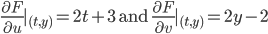
Partial Differential equation (later this semester, used in theoretical physics, e.g. laplace, etc.) u = u(x,y).
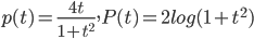
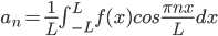
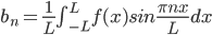
Example:  .
.
Def: The "order" of a DE is the highest derivative that appears.
Example:
Order 1:
y' + y = 0
Order 2:
 There can be many more solutions.
We'll do mostly up to order 2, as most applications do.
Numerical Analysis mentioned. City College supposed to offer this course: Solving problems without formulas.
When initial condition is applied, the solution is called unique solution.
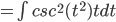
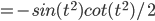
Examples: :
:
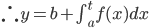
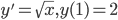
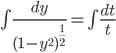
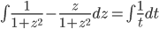
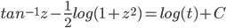
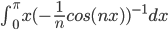
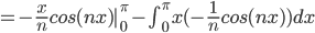
Solve
arctan formula wouldn't work here.
Use 2nd fundamental theorem: Let f(t) be a function and a be a number.
Define "area function":
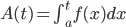
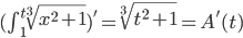
then A'(t) = f(t)
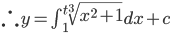
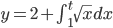
initial condition y(1) = 2
choose a = 1 (easier)
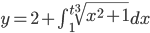
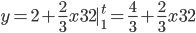
y(1) = 0 + C, so C = 2.
So,
This is the answer. Though unsatisfactory. Computer completes it by use of numerical technique, i.e. Reimann Sum (breaking them into smaller pieces).
In general, to solve y' = f(t), y(a) = b,
Example:
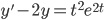
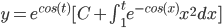
02/03/2016 y' = e^t (also not linear)
First-order linear Differential Equation (FOLDE):
do not mix xy, not linear when the term is a product of x and y.
y
Linear:
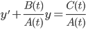
A(t)y' + B(t)y = C(t)
y' + p(t)y = q(t)
Second-order LDE (SOLDE):
A(t)y'' + B(t)y' + C(t)y = D(t)
y'' + p(t)y' + q(t)y = r(t)
for all A(t), B(t), ..., they are coefficients, thus can be squared, etc. and the whole equation can still be linear.
Foundation:

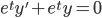


More generally given: "integrating factor"
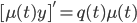
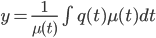

 , such that
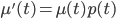
y' + p(t)y = q(t)
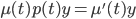
We need to find
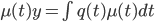
Therefore,
Becomes
Then
need to choose
(log = ln)
But when computing the integral, use a constant to get all functions.
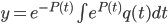
So, to solve y' + p(t)y = q(t)
Example:
ans: p(t) = -2
P(t) = -2t, no need + c since only need one of them
QED
Example:
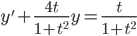
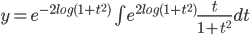


ans:
ans: p(t) = sin(t), P(t) = -cos(t)
Note: by 2nd Fundamental Theorem of Calculus
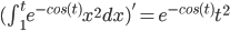


So,
we require
02/08/2016
Dealing with y' = f(t,y), we can solve for y'.
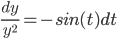
Separable DE has the form
y' = f(t,y) and f(t,y) is separable i.e. f(t,y) = g(t)h(y)
examples:

y' = ty
y' = t + ty
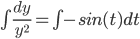
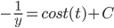
method:

 cause the sqrt to be undefined.
yy' = -t
No global solutions, since when
But there are solutions defined on the interval -1 < t < 1, e.g. when
when 
(Observe that y=0 is a solution, assumption
alternate method (nonsensical way that works, dy/dt manipulation doesn't mean anything except it works, questionable meaning in 1600s - Calculus Pseudomath, used in engineering):
Example:


 this function has no limit.
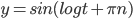
Look for solutions defined for t > 0.
(observe taht y = 1 or y = -1 both solve the DE, so be careful when dividing)
y = sin(log(t)+ C)
This is defined for all t > 0.
But there are no global solutions (except for y = 1, or y = -1) because if we restrict to the domain t > 0, y = sin(log t + C)
and as
Example:
 , t > 0, IVP y(1) = 0;

y = sin(log t + C)
0 = sin(log 1 + C)
0 = sin(0+C)
Therefore,
Where n is an arbitrary integer.
Theoretical D.E. (graduate course) probably not offered at City College, try N.Y.U., email prof. there for free sit-in class.
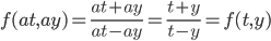
y' = f(t,y), we say f(t,y) is "homogenous" if f(at, ay) = f(t,y)

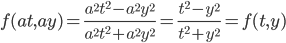
example:
If y'=f(t,y) is given
and f(t,y) is a homogenous function
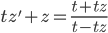
Use substitution
to change DE into separable form.
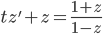
Example:

 , so
, so 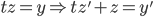

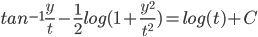
Use
We keep the solution in this form: Implicitly defined function.
02/10/2016
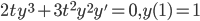
Exact Equation
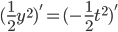
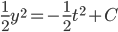
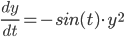
2t + 2yy' = 0 (not linear, but separable)
2yy' = -2t
y' = -
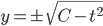
Another method: = 0
= 0


=
This differential equation is called "exact" i.e. the DE can be expressed as an exact derivative.
Let F(u,v) be a function of two variables.
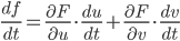
Subtitute u = g(t) and v = h(t)
Form the composition F(g(t),h(t)) = f(t)
Example:
(2t+3) + (2y-2)y' = 0
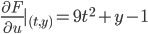
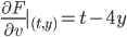
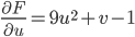
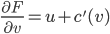
We need to find a function F(u,n) so that
Therefore,


F(u,v) has to satisfy:
Therefore,

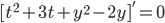
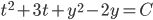
(implicit solution)
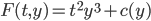
Example:
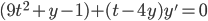


We try to find a function F(u,v) so that,
So,
We found
So,
Example:


(this is actually linear)
Choose c(y) = 0
Thus,
So the E,
evaluate at t = 1;
so c = 1.
Example that does not work:


 but
but 
y + y' = 0
Try to find F(t,y) so that
F(t,y) = yt + c(y)
so,
t + c(y) = 1, which is not possible to find the F(t,y) this way. The equation is not exact.
Conditions:
An equation of the form
M(t,y) + N(t,y)y' = 0
is called "exact" if we can find F(t,y) so that [F(t,y)]' = M(t,y) + N(t,y)y'
How do we know if that equation is exact?

Cross-partial test (prof.'s made up term)
02/17/2016 (IVP)
(IVP)
(Today's lesson Not on Department Final)
(Emilie) Picard's Theorem (systems of DE):
Given y' = f(t,y), with
There exists a unique solution.
Consequence 1:
Given y' = f(t,y)
if y = c (trivial) is a solution, then any other solution is never equal to c.
Example:

 will never be equal to 0.
Given
Observe that y = 0 solves the DE. So any other solution
Consequence 2: and
and  are two different solutions then they never intersect.
Given the DE y' = f(t,y)
If
y' = y

The solutions are given by
Euler's Method

A numerical method for approximation the solution of the IVP
Linear Approximation
Autonomous Equations

 (not autonomous)
DE of the form
y' = g(y)
examples:
y' = y
Note, Autonomous DEs are separable, and so can be solved by separation of variable technique.
Def: Trivial solutions to an autonomous equation ie. y = c (constant solutions) are called "steady state solutions".
Example: y' = (1-y)(y-2)
SSS are of the form y=c,
0 = (1-c)(c-2)
c = 1, 2
Thus, S.S.S. are y = 1 and y = 2.
Claim y'(t) > 0 for every t. = 0.
= 0.
Otherwise there will be some point in time to such that
Example:


Determine
log(sec y + tan y) = t + c
first find the s.s.s.
let y = c,
0 = cos(c)
y'(0) = cos(y(0))
=
02/22/2016
Population growth
(not covered by Department)
Let y(t) be the population size at time t.


Then Rate of growth (y'(t)) is Directly Proportional to Population Size (y(t)).
Simple Exponential Growth(useful only when dealing with small populations - e.g. death not accounted for)/Malthus Model:
y' = ry
The stead-states of y' = ry are only y'=0.
How we arrive at the equation:

FOLDE:
y' - ry = 0
p(t) = -r
q(t) = 0
P(t) = -rt
Example:
Initially a population size consists of 10,000 cells.
After 2 hours the population size is 30,000
What is the population in the next hour?
Ans:
Let y(t) = pop. size measured in 10,000's, at time measured by hours.
y = y_e^{rt}
so y = 1\cdot e^{rt}
y(2) = 3
so
We want y(3) = ?
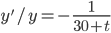
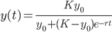
Verhulst Model:
y' = r(y)y
Suppose that the population has "carrying capacity" = K
y' = r(1-y/K)y
Look for steady-state solutions y = C
So, 0 = r(1-C/K) C
C = 0, K
y'(0) = r(1 - y(0)/K) y(0)
Thus, the rate in increasing.
Now find the inflection point:


Inflection occurs at
so, y = K/2
Always concave up first, passing inflection point, then concave downward.
Hence, a Logistic Function.
When is the rate of growth increasing most rapidly?
Optimize y'
Juxtapose simple exponential function with logistic function, it shows that it is not much problem using simple function before the inflection point.
Solve: y' = r(1-y/K)y
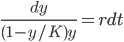
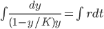


dy/dt = r(1-y/K)y
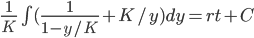
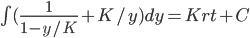
Do partial fraction (prof's guessing method)
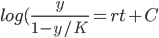
K log(y) - K log(1-y/K) = Krt + C
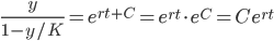
log(y) - log(1-y/K) = rt + C
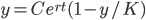
Make it more aesthetic:
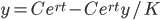
multiply by
02/24/2016
 (r will be negative)
Law of Cooling
The rate of cooling, y'(t), is dir. prop. to the change in the temperature, y-T.
solves the DE.
Example:
Vodka is 20C. Refrigerator is at -10C. It is placed in the refrigerator and 10 minutes later its temperature is 15C. When will the Vodka reach 0C?
let y(t) = temperature of Vodka at time t.


Since y(0) = 20,
C = 30.
Thus,
y(10) = 15
Solve,
y(t) = 0
Example:
Tank has 30 liters of liquid, which consists of water and 10 pounds of salt dissolved in it.
Liquid is pouring in at the rate of 2 liters/min and contains 1 pound of salt.
There is a hole at the bottom of the tank, liquid is pouring out at the rate of 2 liters/min.
After 1 hour how much salt is in the tank?
y(t) = amount of salt at time t, inside the tank.
y' = rate of change in salt = rate in - rate out = 1(per minute) -
Concentration = weight/volume
at time t, the concentration of salt in the tank = y/30
y' = 1-y/15, y(0) = 10
 .
.
y' + y/15 = 1
p(t) = 1/15
q(t) = 1
P(t) = t/15
thus, C = -5.
y(60) = ...
lim y(t) = 15
Example:


Tank has 30 liters of liquid, which consists of salt water having concentration 2 lbs/lit of salt.
Pure water is pouring at the rate of 2 liters/min.
There is a hole at the bottom of the tank, liquid is pouring out at the rate of 1 liter/min.
Set up DE for the amount of salt at time t.
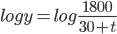
(log y)'= (- log (30+t))'
log y = log(30+t) + C
y(0) = 60
log 60 = -log(30) + C
C = log 1800
log y = -log(30+t) + log 1800
Logistic Equation
y' = r(1-y/K)y
r = growth rate
K = carrying capacity
Example: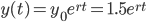


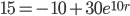
A lake initially contains 15,000 fish, and carrying capacity for the lake is 300,000 fish.
In the first few years the fish increase in population at about 10%.
When will the population reach 200,000 fish?
Ans:
y(t) = amount of fish measured in 10,000 units.
y(0) = 1.5
If y(t) is "small" then
y(1) = 1.65
Logistic equation:
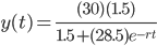
Solve, y(t) = 20.
02/29/2016
Second Order Linear DE
a(t)y'' + b(t)y' + c(t) y = f(t)
Assume a(t) is not 0,
we will deal with:
y'' + p(t)y' + q(t)y = F(t)
Off-topic:
Galois at 20, proved quintic equation not possible, died next day.
Hence, study of Galois Theory.
y'' - y' = 0, let z = y'
z' - z = 0
z = Ce^t
y' = Ce^t
y = Ce^t + d
Example:
y'' + y'/t - y/t^2 = 0, t > 0
(y' + y/t)' = 0
y' + y/t = a
p(t) = 1/t
q(t) = a
P(t) = log t
Theorem: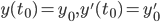
Given a SOLDE:
y'' + p(t)y' + q(t)y = f(t)
together with IVP
There exists a unique solution.
(proven in high level DE)
If f(t) = 0, this is a simplified DE which we call "homogeneous".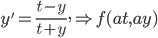 , etc.
Note:
Not the same kind of homogeneous as:
If equation is homogeneous in SOLDE:
i) If y is a solution to such a DE, then cy is also a solution.
ii) If y_1 and y_2 are solutions tot he DE, then y_1 + y_2 is also a solution.
Consequence:
ay_1 + by_2 will solve the DE.
Example:


y'' - 3y' + 2y = 0, y(0) = 1, y'(0) = 0
Guess a solution of the form
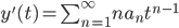
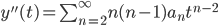
So, y' =
y'' =
Choose k such that:
k = 1, 2
So, and
and  are solutions.
 is also a solution
Since this DE is homogeneous,
To determine a = ?, b = ? use the IVP.
Determinant of (2x2, our focus) ,
,
 = 4+3 = 7
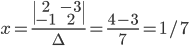
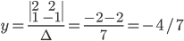
Application example:
2x - 3y = 2
x + 2y = -1
Only when
This works for n x n matrices as well.
Gauss-Jordan Elimination: the fastest method for solving system of linear equations.
03/02/2016 and
and  solutions to the DE then
  will solve the DE, provided that the DE is homogeneous.
SOLDE has the form:
y'' + p(t)y' + q(t)y = f(t)
i) Given an IVP y(t_0) = y_0 and y'(t_0) = y_0' there exists a unique solution (Main Theorem)
ii) If f(t) = 0, then we call this equation "homogeneous".
iii) given
GIven a HSOLDE: y'' + p(t)y' + q(t)y = 0 are "dependent" if
 (these are dependent)
We say two solutions
Example:
Otherwise they are "independent" solutions.
Example:
Another formulation of what it means for y1 & y2 to be dep/indep.
If the only way the expression c1y1 + c2y2 can be made equal to zero is when c1 = 0 and c2 = 0 then y1 and y2 are independent.
Example: Let y1 and y2 be solutions to a HSOLDE.
To check that y1 & y2 are independent, we have to show that the only way c1y1 + c2y2 = 0 is only when c1 = 0 and c2 = 0.
If determinant is not 0, then c_1 = 0, c_2 = 0. Thus, y1 & y2 are independent.
Def: Given two solutions y1 and y2,
the "Wronskian" of y1 and y2, denote it by W(y1, y2)
W(y1, y2)(t) = determinant =
Theorem: Given a HSOLDE, with y1 and y2 two solutions.
IF there exists a number t_0 so that W(y1, y2)(t_0) != 0
then every solution of (*) has the form c1y1+c2y2.
In other words, if y3 is another solution then y3 = c1y1 + c2y2, for some choice of c1 and c2.
Proof:
Let y3 be a solution of (*)
Find constants c1 and c2 so that,
c1y1(t_0) + c2y2(t_0) = y3(t_0)
c1y1'(t_0) + c2y2'(t_0) = y3'(t_0)
This is possible, != 0.
!= 0.
Observe that c1y1 + c2y2 and y3 satisfy the same initial-values at t_0.
But, by uniqueness (Main Theorem), these must be the same, y3 = c1y1 + c2y2.
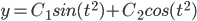
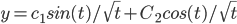
Example: every solution to y'' + y = 0 has the form: c1*sin(t) + c2*cos(t) => y3
Def: Given a HSOLDE,
we call a pair of solutions y1 and y2 a "fundamental pair" if W(y1, y2)(t_0) != 0, for some t_0.
Example: y'' - y = 0
e^t and e^{-t} is a fundamental solution pair, so every solution is of the form c1e^t + c2e^{-t}
but, cosh(t) and sinh(t) is also a fundamental pair, so every solution is of the form, c1cosh(t) + c2sinh(t). But all the fundamental pairs are really equivalent.
Theorem:
Every HSOLDE has a pair of fundamental solutions.
03/07/2016 != 0, for some t_0, then every solution of the DE has the form
  .
.
Review: Given a SOLDE homogeneous:
y'' + p(t)y' + q(t)y = 0
with y_1 and y_2 solutions.
We call y_1 and y_2 a "fundamental pair":
If
Abel's Theorem: Let W = W(y1,y2), then W' + p(t)W = 0


Prove:
thus,
1st Consequence: since the theorem looks like FOLDE,
2nd Consequence: W(t) is either identically zero, or else, nowhere zero.
Question:
Have we covered finding fundamental pairs when W is zero?
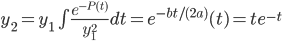
Let us say that we have HSODE, and we happen to know that y_1 is a solution,
 is actually =
can we somehow find a y_2 so that y1 and y2 will form a fund. pair.
Note:
Thus,
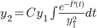
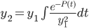
3rd Consequence: If we have y1, we can find y2 so that y1 and y2 form a fund. pair by choosing
Example:
 , given that


Solve the DE.
p(t) = -1/t, thus, P(t) = -log t
Instead we can even choose
Then, the solution is:
Prof: Another method (Reduction of order: Dalem Bear's method?) mentioned in book to solve for y_2.
Example: Solve y'' - 2y' + y = 0, given that y1 = e^t is a solution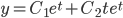
Ans: y_2 = te^t
Hence,
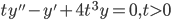
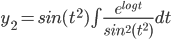
Example: t^y'' + ty' + (t^2-1/4) y = 0
 is a solution
Solve the DE
(This is Bessel's equation)
Ans:
Thus,
03/09/2016 .
.
Non-homogeneous SOLDE:
y'' + p(t)y' + q(t)y = F(t)
Method:
1. First find a fundamental solution pair for the homogeneous equation, call them y1 and y2.
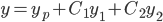
2. Find a "particular solution" to the non-homogeneous equation and call it
3. All solutions to the non-hom. DE are
#3 works because: solves the same equation then
  will solves the HSOLDE.
If y solves the non-HSOLDE, and
So,
Example:
y'' - 2y' - 3y = 3e^{2t}
Check that y_p = -e^{2t} then theis solves the DE.
So this is a "particular solution".
Check that -e^{2t}+e^{-t} also solves the DE.
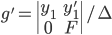
LaGrange:
Start with the DE, y'' + p(t)y' + q(t)y = F(t)
Look for a y_p of the form:
Wishful thinking: exists
First,
Second,
Thus,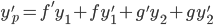
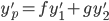
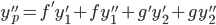


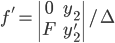
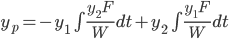 , where
Thus,
Since y1 & y2 are pairs for homogeneous equation,
1)
and we already have:
2)
This is called "Variation of parameters"
Example: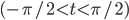


y'' + y = tan t,
First find a fun. pair to the HSOLDE: y'' + y = 0
Pick y1 = sin(t) and y2 = cos(t)
y_p = -sint(cost) + cost(-log(sect+tant)+sint) = -cost(log(sect+tant))
Thus, the solutions are given by:
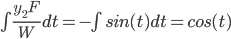
Example: Solve


Ans: W = -3
Example: Solve


y_p = sin^2t(t^{-1/2} + cos^2t(t^{-1/2} = t^{-1/2}
Thus, Solution to the DE is:
03/14/2016
Solving the DE:
ay'' + by' + cy = 0
Look for solutions of the form:


 , solve for k.
 and
and  form fun. pair
 and
and 
 will solve the DE.
 , then


 form the fun. pair
Thus,
There will be 2 solutions for k, which in turn gives fundamental pair solutions for y.
To solve ay'' + by' + cy = 0,
write down "characteristic polynomial": ax^2 + bx + c, find the roots (zeros)
i) If there are two roots u and v, then
ii) If there is only one root, q, then
Why? The root in quadratic formula is = -b/(2a), and b^2-4ac = 0.
Then,
from y'' + by'/a + cy/a = 0 => p(t) = b/a, => P(t) = anti-derv. of p(t) = bt/a
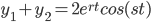
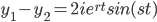
iii) If complex roots
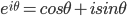
Euler's Identity:
Fun note: Euler was later blind. 76 volumes of work, some has not yet been translated from Swiss.
Hamilton's quaternion imaginaries mentioned. Used for computer graphics.
then
Solve, y'' - 3y' + 2y = 0: solve the DE and form a fun. pair.
x^2-3x+2=0
(x-1)(x-2) = 0
roots 1 and 2
Thus,
Then,
Solve, y'' + 2y' + y = 0
root: -1 (with multiplicity 2)
Thus, y_1 = e^{-t}
Solve, y'' + y = 0 where r = 0, s = 1


x^2 + 1 = 0
root =
y'' + y' + y = 0
roots:
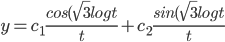
To solve Euler's Equation: , (Euler-Cauchy Equation)


 and
and 
 and
and 
 are complex roots use
(Prof. noted that he couldn't find an application for this equation)
Form the "char. poly.": ax(x-1) + bx + c
How: Look for solutions of the form
plug in to the equation and we get:
Need to solve, ak(k-1) + bk + c = 0, thus, the "char. poly."
i) If u and v are roots then use
ii) If u is the only root then use
Almost in the Department final exam
iii) If
Solve,


1x(x-1) + 3x + 4
roots:
03/16/2016
A(t)y'' + B(t)y' + C(t)y = 0
Were the coeficients are polynomials
We say this DE is "regular" (good in mathematics) if A(0) != 0
Otherwise the DE is "singular" (bad) i.e. if A(0) = 0
In the regular case we can solve the DE with a power series
Thus,
plug these into the equation.
A analytic function: one that can be written in power series.
Example: with recurrence relation.
 .
. and
and  in power series form is fine in exam.


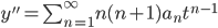
y'' -2ty' + 4y = 0
Turn y into power series, manipulate initial term, n, and necessary variables in such a way they can be combined.
Then, force all partial groups of terms to 0.
Solve for
This gives the coefficient for
Writing
Example:

y'' - ty = 0
03/21/2016
Exam, note power series solutions in SOLDE
We did "regular" DE
Now let's see "singular" DE
Supposed A(0) = 0 and we can write:
 , where a(0) != 0
B(t) = tb(t)
let a(t) =t+1
Thus,
this is called "regular singular", since a(0) != 0.
Look for solutions of the form y =
Recall characteristic equation
Where the power p is a root of the polynomial:
a(0)X(X-1) + b(0)X + C(0)
(Frobenius Method)
Look in book for explanation (off topic)
Example:
ty'' + y = 0
multiply t to eq:
Thus, X(X-1) + 0X + 0 = 0
roots = 0, 1
Technically, all roots must be solved.
first, look at root = 1
Look for a solution of the form
solve recurrence relation:
Thus this solves for the larger root.
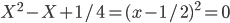
Example:

This DE is singular (but regular singular)
It should remind us of the Euler Cauchy form
X(X-1) + 0X + 1/4 = 0
Look for a solution of the form
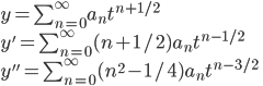
plug them into equation and get similar exponents
then, replace n by n-2
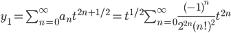
Thus, we make coefficients of t be zero:
accepted answer
further simplification:

03/30/2016
Higher order DE will not be taught in class, but in HW and exam.
Today:
Vibration
Prereq: Hooke's Law (Robert Hooke 1635-1703) invented microscope and word "cell".
The displacement of a "spring" from its natural length is directly proportional to the force.
Force/Displacement = spring constant or elasticity "constant".
Works on rubber bands too, but rubber bands cannot be compressed.
The reason for vibration: when things are elastic.
y(t) = position of the mass measured from its equilibrium, from equilibrium due to Hooke's Law.
equilibrium (distance when object is motionless)
y'(t) = speed
y''(t) = acceleration
Hence, most DE order up to 2.
Higher order than 2 application in the Beam problem.
The sum of all the forces acting on a body = ma (the reason subway riders fall when taking a seat)
Newton's law = Hooke's law, eventhough they disliked each other , y'(0) = 0
ma = -ky
my'' = -ky
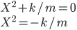
y'' + ky/m = 0
y(0) =
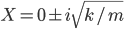
Solve:
I thought that perpetual motion is not possible, hence this knowledge is just for foundation purpose, I supposed.
Thus,
The amplitude of the vibration =
Period of the vibration =
Take note on this Final Exam sample:
A spring has NL 10 in, and elasticity = 2 lbs/in
A mass is attached to the spring, of the weight 10 lbs.
Pull the spring to 13 in, we push towards the wall at 1 in/sec.
Determine the amplitude and the period of this vibration.
Ans:
y_0 = 3
y'_0 = -1
k = 2
m = 10/32
10y''/32 = -2y
5y'' + 32y = 0
y'' + 6.4y = 0
y(0) = 3
y'(0) = -1
y(t) = 3cos(.8t) - 1.25sin(.8t)
period =
Why metric system? Because every type of unit is defined by another metric type. Easier.
y = Asin(t) + Bcos(t)
amplitude:
Damping force = the amount of force per speed.
The damping force is directly proportional to speed
10y''/32 = -2y - 0.1y'
04/04/2016
Numbers --- functions ---> numbers
Functions --- transform ---> functions
example: d(f(t))/dt = f'(t)
Let f(t) be a function defined for t>= 0
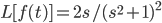
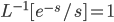
The "Laplace Transform of f(t)":
~f(s)
Domain of ~f are all values of s for which the int. converges.
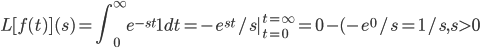
example: f(t) = 1
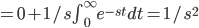
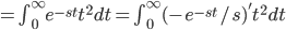
example: f(t) = t
draw graph
again, no need to care what function does for negative value
L[t](s) = \int^\infty_0 e^{-st}t dt

Integration by parts
easier way to do:
Example:

Thus,


Table:
f(t) | ~f(s)
1 | 1/s
Example: f(t) = t, if t is zero to 1, 0 if t > 1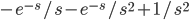
Do int as if 0 to 1.
ans:
limit rule of Laplace Transform: ) = 0
) = 0
~f(+
Compression Rule:
Say f(t) has Laplace transform ~f(s)
L[f(at)] = 1/a * ~f(s/a)
a > 0
Example: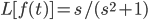
find
Rule:
L[f(t)+g(t)] = L[f(t)] + L[g(t)]
L[af(t)] = aL[f(t)]
Linear mapping of bounded functions of exponential growth
Example: L[3t^3 - t^2 + 4] = 3*3!/s^4 - 2!/s^3 + 4/s, too easy to be on exam
Origin of Compression Rule, proven. Easy.
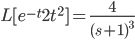
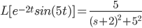
Shift Rule:
If L[f(t)] = ~f(s)
then L[e^{at}f(t)] = ~f(s-a)
Example: Find L[e^t * t](s)
L[t] = 1/s^2 = ~f(s)
ans: ~f(s-1) = 1/(s-1)^2
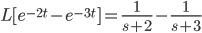
Exponent Rule
L[e^{at}*1] = 1/(s-a)
Example: L[e^{-2t}] = 1/(s+2)
Exam
Median: 84
Highest: 112
Lowest: 9
1/3 failed
1/5 over 100
Review of Laplace rules:
Limit, Compression, Shifting, Delay
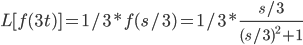
Additional Laplace Rule:
Delay:
Prove: let u = t-a, ...
Find: L[(t^2+1)e^t]
sol:
L[t^2+1] = 2/s^3 + 1/3, using table and linear rule
L[(t^2+1)e^t] = 2/(s-1)^3 + 1/(s-1)
Find: L[cos t] = \int^\infty_0 e^{-st} cos t dt
Could use integration by parts and solve for I.
But smarter way:
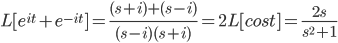
Euler's identity: e^{it} + e^{-it} = 2cos t
So,
New rule:

f(t) = cos t
f(at) = cos(at)
New rule: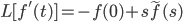

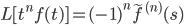
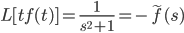
Derivative Rule I:
Origin:
For f(at) = sin(at)
f(t) = cos (at)
f'(t) = -a sin (at)
L[f'(t)] = -f(0) + s\tilde{f}(s) = -1 + s\frac{s}{s^2+a^2}
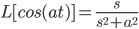
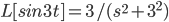
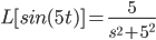
L[sin(at)] = \frac{a}{s^2+a^2}
So, we have table for
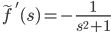
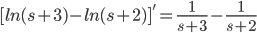
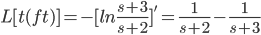
Derivative Rule II
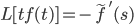
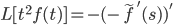
Origin:
Differentiate both sides of formal L equation.
push d/ds on RHS into content of integration.
That is called Leibniz rule of differentiation(?), Rich Feynmann said it's the only trick in derivative.
Find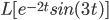

So, ans:
Find
 first.
Found by solving
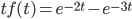
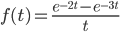
Find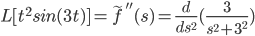
Example:
 = ?
= ?


f(t) = sint/t
tf(t) = sin t
Since
04/11/2016
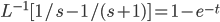
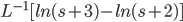
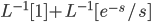
Inverse Laplace Transform:
theorem (uniqueness): If f(t), g(t) are continuous functions and L[f(t)] = L[g(t)]
then f(t) = g(t)
Given a function g(s), to be a function f(t) so that L[f(t)] = g(s)
denote by
Example:
We had formula for Laplace transform, the inverse is called: Mellin-transform
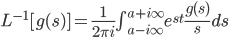
Example: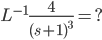
Example:
(no theorem for product-look up convolution, but for sum)
In Engineering: Convolution (not used in class)
L[f(t)*g(t)] = L[f(t)]L[g(t)]
Example: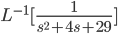
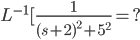

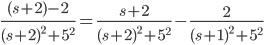
Irreducible quadratic (complex roots)
Use "completing the square"
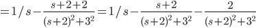
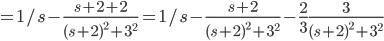
ans:
Example: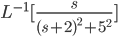

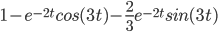
Ans:
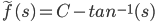
Example:

try integrate it
integrate
Example:
So,
Example: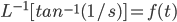

L
tf(t) = sin t
Example:

 for
for  ; 0 for t < 1
 : graph shift up 1 unit.
Use delay rule
L[f(t)] = 1/s
Do the following when applying delay rule:
Example: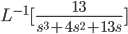
Get partial fractions
Ans:
04/13/2016
Use Laplace Transform to solve DE
y' + y = 0


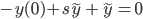
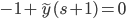

y(0) = 1
Use Laplace instead:
L[y'+y] = L[0]
L[y'] + L[y] = 0
Example:


Normal solution: use Wronskian
Use Laplace:
Do partial fraction on first term on RHS
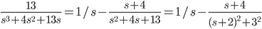
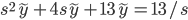
Example: y'' + 4y' + 13y = 13, y'(0) = 0, y(0) = 0
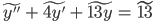

y = done in last class
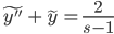
Example:
 , root has multiplicity 4.
Ordinary method:
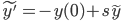
Laplace:
(-y'''(0) - sy''(0) - s^2y'(0) - s^3y(0) + s^4\tilde{y}) - \tilde{y} = 0
1 - s + s^2 - s^3 + s^4\tilde{y} - \tilde{y} = 0
(s^4-1)\tilde{y} = s^3-s^2+s-1
\tilde{y} = \frac{(s^2+1)(s-1)}{(s^2-1)(s^2+1)} = \frac{1}{s+1}
y = e^{-t}
If initial parameters is not 0, then try delay rule. But test will use 0.
Fourier Series: When dealing with periodic function

Optional (Fourier Transform)
simplest functions with period 2pi: sin(), cos(), 1, etc.
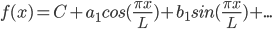
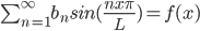
Given a function f(x) of period p, (where L = half-period), try to write f(x) as infinite series:

Example:
f(t) = sin(at)
What is the period? 2pi/a
f(t+2pi/a) = f(t)?
Yes.
sin(nat), cos(nat) has period 2pi/a
p = 2pi/a, L = 1p/2
04/18/2016
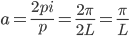
Fundamental Period: 2pi/a
It also has periods = 2npi/a, n is positive integer
f(x) = sin(ax)
f(x+2pi/a) = f(x)
sin(a(x+2pi/a)) = sin(ax + 2pi) = sin(ax)
Let L = p/2
p = 2pi/a
a = 2pi/p = 2pi/(2L) = pi/L
sin(xpi/L) and cos (xpi/L) have periodic = p
sin(xnpi/L) and cos(xnpi/L) have period = p
2pi/(npi/L) = p/n
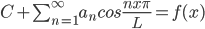
Let f(x) be a periodic fun. of period p i.e. f(x+p) = f(x)

Try to express f(X) in the following form:
C is also periodic.
note n & m
if n = m, it is equal to L
cosine equivalent formula also.
The above are orthogonality relations
expand f(x)
 , everything else is 0.
to get C, integrate equation from -L to L.
thus,
To find a_2, multiply f(x) equation with the function next to , thus,
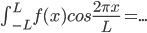


every terms on RHS is zero due to orthogonality relations except one:
Thus,
Alert: these are based on infinite series assumption.
Let f(x) be a periodic fun. of period p. Let L = p/2

The "Fourier series of f(x)" is:
But not proven until recently, "Carlsen's theorem?"
However, not all power series = Taylor's series.
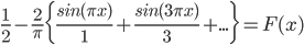
Example: "Sawtooth Wave" function

f(X) = x if -pi < x \leq pi
f(x+2pi) = f(x)
these two describes a full graphs.
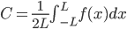
C = 0 = \frac{1}{2\pi} \int^{\pi}{-\pi} f(x) dx =
Note:
Even function, E(-x) = E(x)
Odd function O(-x) = -O(x)
odd * even = odd, this is about functions, not numbers
Hence, integrate cosine in this case is 0.


Easiest way of integrating by parts:
thus,

Thus, since Fourier Series of
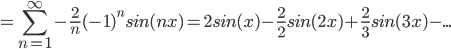
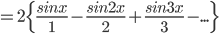
and the answer:
F.S.
04/20/2016
Exponential Growth not on Final Exam.
Recap:
 where
where 

Let f(x) be a periodic function of period p:
The "Fourier Series" of f(x) is the series:
We are going to ask is f(x) = F(x)
Graph:
test it with partial sums.
This is F(x) built from graph.
Dirichlet Convergence Theorem
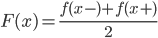
If f(x) is continuous, then F(x) = f(x)
Example:
let f(x) = x^2 for -\pi \leq x \leq \pi
and give f(x) period = 2\pi
graph it.
C = \pi^2/3
b_n = integral of even function (x^2) and odd function (sin(nx)) = 0
a_n = \frac{2}{\pi} \int^{\pi}_0 x^2 cos(nx) dx, integrate by parts = \frac{4}{n^2}(-1)^n
f(x) = \frac{\pi^2}{3} + \sum^{\infty}_{n=1}\frac{4}{n^2}(-1)^n cos(nx)
Let x = \pi;
\pi^2 = \frac{\pi^2}{3} + \sum^{\infty}_{n=1} \frac{4}{n^2}(-1)^n(-1)^n
\frac{2\pi^2}{3} = \sum^{\infty}_{n=1} \frac{4}{n^2} \Rightarrow \frac{\pi^2}{6} = \sum^{\infty}_{n=1} \frac{1}{n^2}
05/02/2016
 = periodic & odd extension of f(x).
 for
for 
 if
if 
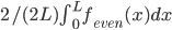
Let f(X) be a function defined for
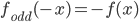
find the "sine series" of f(X).
Thus, function has to be odd (even for cosine series)
Define
Note:
side note:
Find the Fourier series of


 Provided that f is continuous and f(0) = f(L) = 0.
C = 0
Then the "Sine Series" of f(x):
Now let's do cosine series of f(x). = periodic extension of f(x)
 from 0 to L
 has period = L, so 2L, any multiple is also period.
 = replace
  with
with 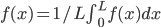
 = even integral * even (cosine) = not zero =
 = 0 (even * odd?)
 provided that f is continuous.
Define
Note
Find the Fourier series of
C is not 0, thus, integrate it =
Thus, the cosine series of f(x) =
Where
Example:
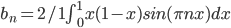


let f(x) = x(1-x), define on the interval
Find its Sine Series
lots of int by parts.
Prof's way:
do another int by parts, prof's method:
thus, b_n = 0 if n is even, \frac{8}{\pi^3 n^3} if n is odd
Not complete yet,
Thus, in Fourier series:
(\sum^{\infty}_{n=1} (-\frac{4}{\pi^3 n^3}((-1)^n - 1)) sin(\pi nx)
good enough, but can also try to expand the series.
05/04/2016
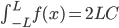
Heat equation always in Final
Heat equation:


(PDE condition)
or simply:
Where u(x,t) = heat at x at time t.
f(x) = initial heat at position x, => u(x,0) = f(x), (IVP condition)
thus, u(0,t) = u(l,t) = 0, (BVP, boundary value problem)
The solution to the conditions:
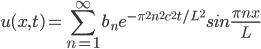
 is the sine series coefficients of f(x)
This equation is known as Fourier's method
Check if the equation satisfies the above 3 conditions.
f(x) will be the sine series.
If both ends are insulated, then f(x) is from cosine series instead.
Example:

Solve:
u(x,0) = 1, => uniform heat
u(o,t) = u(2,t) = 0.
Solution:


f(x) = 1
Since, L = 2
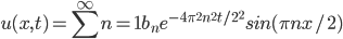
Example:
u(x,0) = sin x - 2sin (3x) = f(x)
u(0,t) = u(1,t) = 0
Thus,
done
05/09/2016
Exam II:
1 Question on Oscillation.
3 Questions on Laplace transform, (1 solve DE using transf., 1 invert transf., compute/find using transf. Laplace)
1 Find Fourier/sine/cosine series
1 heat equation
1 solve higher order eq with const. coefficient (solve by finding 2nd order...)
1 Method of Undeterminded Coefficients (Prof. a waste of time)
Do 4 out of 8.
Method of Undetermined Coefficients:
Given ay'' + by' + cy = F(t)
Find y_p (particular solution), already taught.
For Exponential:
y'' + y = e^t
so, X^2 + 1 = 0 => roots: 0 \pm 1*i
y_1 = e^0cos(1t) = cos t
y_2 = e^0sin(1t) = sin t
The method:
guess y_p = Ae^t = y'_p = y''_p
Ae^t + Ae^t = e^t
2Ae^t = e^t
A = 1/2
y_p = 1/2 * e^t
y = c_1 cos(t) + c_2 sin(t) + 1/2 * e^t
solve: y'' + y = e^{2t}
4Ae^{2t} + Ae^{2t} = e^{2t}
5A^e{2t} = e^{2t}
A = 1/5
y_p = 1/5 * e^{2t}
...
For Polynomial:
y'' + y = t^2
guess y_p = At^2 + Bt + C
For ...:
y'' + y = sin(2t)
guess y_p = Asin (2t) + Bcos (2t)
y'_p = 2A cos(2t) - 2B sin(2t)
y''_p = -4A sin(2t) - 4B cos(2t)
So, in y'' + y => -3A sin (2t) - 3B cos (2t) = sin 2t, A = -1/3, B = 0
Example:
y'' + y = e^t cos t
Guess y_p = e^t (A sin t + B cos t)
Example:
y'' + y = sin t
Problem for guess y_p = (A cos t + B sin t)t
Example:
y'' - 2y' + y = e^t
X^2 - 2X + 1 = (X-1)^2
y_1 = e^t, y_2 = te^t
Guess y_p = Ae^t won't work
y_p = tAe^t still won't work
y_p = t^2 Ae^t works.
05/11/2016
Final May 23rd, 1pm, NAC 0/201
population growth & Euler's method not on Final
Need to know formula for a^3 - b^3 = (a-b)(a^2+ ab + b^2)
X^3+1 = (a+b)(a^2- ab + b^2)