
Professor: Peter Brass, NAC 8/208, office hours: Wed 3-4pm; email: peter@cs.ccny.cuny.edu, phjmbrass@gmail.com (homework submission)
4 HW projects: each implementation of an algorithm in C/C++
Interface & test code provided, submission must pass on prof's computer. No partial Credit - (pass/fail only).
Recommended reading: Kernighan/Ritchie's The C Programming Language.
Recommended compiler: gcc/g++
Grading:
median of (HW, midterm, final) + adjustments (positive for early HW submission; negative for too many resubmissions, resubmission without fixing, does not compile) = course grade.
To get A: 1) pass 4 HW and either A in Midterm or Final; Or 2) pass 1 HW and A in both midterm and final. All tests are open book (printouts only, no laptop).
Lookup algorithms in Wikipedia. Everything in there.
Sorting n numbers:

Given n numbers in an array, we want to sort them in increasing order so:
Bubble Sort Algorithm
idea, sample run, code, runtime (worst case scenario/upper bound).
two loops.
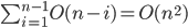
Outer loop runs at most n times.
Inner loop takes n*c time of test and exchange.
Upper bound for bubblesort for array of length n is runtime < c * n^2, where c is time of test-and-exchange.
How many exchange operations do we need in the worst case?
call (i,j) a transposition of array a[] if a[i]>a[j] and i < j.
Each exchange in bubblesort (two neighboring elements) decreases number of such wrong pair (i,j) by one, if we start with a decreasing sorted array then all pairs (i,j) with i < j are wrong pairs.
 such pairs =
  , so time required to sort decreasing array into increasing order by bubblesort
  , where
  is time of exchange.
there are length n with runtime > c_1 * ~
~  , where
  is time of exchange.
02/03/2016
Asymptotic Analysis / O-Notation
(Landau symbols)
Define some abbreviations
1) f(n) = O(g(n)) is abbreviation for
 g(n)
g(n)
There is a constant C such that for all n, f(n) < C
f, g are assumed to be positive.
2) is abbreviation for,
there is a constant C > 0, such that for all n
3) is abbreviation for
 such that
there are constants
4) f(n) = o(g(n)) is abbreviation for such that for all
for all C > 0, there is an
5) is abbreviation for
 such that for all
for all C, there is an
Comparing two explicitly given functions: exists and is <
 , then f(n) = o(g(n))
if
then f(n) = O(g(n))
if limit
if limit exists and is > 0, then
If f(n) = O(g(n)) and g is increasing


 , are summands of all
then
Why?
where n in
Selectionsort / Insertionsort
Incremental sorting: we maintain a sorted part of the array and add new elements at the right place
Insertionsort: Want to sort array a[]
maintain sorted part a[0]...a[i-1]
Insert a[i] in the right place, shifting everything behind it backward.
Analysis of insertionsort:
The inner loop shifts at most i element, so takes O(i).
Outer loop runs i=1...(n-1)
so total time is
Selectionsort idea:
Want to avoid shifting the elements of the sorted array.
We can do this by the right choice of the next element:
if we always insert at the end, we don't have to shift.
So - first find the largest element, put it in last place, then find second largest, put it in the second last place...(prof's method)
Analysis: runtime
We saw three different algorithms,
 for some input arrays
each solves in
and reads
For testing a sorting function you want to generate an array which is "mixed" but you know what it should be after sorting.
Select p prime, constant b, then (i*b) mod p for i = 0...p-1
is a permutation of 0, 1, ..., p-1
02/08/2016 2 * time(n/2) + O(n)
Fast Sorting Methods I: Mergesort
Idea: Divide and Conquer
Divide our input array in two (halves), takes O(1), sort each separately <- Recursive Call, takes 2 * time(n/2)
merge the sorted arrays, takes O(n).
Recurrence Relation for the runtime time(n)
Merging two sorted arrays of combined length n takes O(n) time.
repeat until one array is empty,
compare first element of both arrays
move the smaller to the output array
then move the rest of the other array to the output array.
Prove Bound for runtime using INDUCTION C n log n
 2 time(n/2) + O(n)
 2 time(n/2) + Bn,
Want to show: time(n) = O(n log n)
means there is a C such that time(n)
We have: time(n)
means there is a B such that time(n)
B is given, C we can choose
Want to show: time(n) C n log n for some C(we choose)
 2 time(n/2) + Bn (B given)
 C k log k
 C (n/2) log (n/2) = C(n/2)log(n) - C(n/2)log2
 2(C(n/2)log(n) - C(n/2)log 2) + Bn = Cnlog(n) - Cn log 2 + Bn
 B, then -Cn + Bn
  0
0 Cn log(n)
Have: time(n)
Proof by induction: Assume we have already for all k < n
time(k)
then time(n/2)
(log taken to base 2, so log 2 = 1)
So time(n)
Choose C
So time(n)
So, mergesort needs O(n log n) to sort n numbers.
Exercise: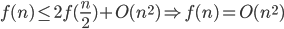

 , we choose A
 for k < n
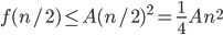


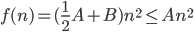
Show
Ans:
We have:
we want:
Inductive Assumption:
then
So,
Choose A such that
Mergesort without recursion: Breaking array into two (even side and odd side), back in the classic Fortran day.
When system restrict memory usage, look into: ulimit -s unlimited
02/10/2016
Prof. called us to go for CUNY Math Challenge.
In the fall there will be ACM programming Contest: International Collegiate Programming Contest
Look at UVA Problem Archives if interested (link?).
Quicksort
idea: Randomized Algorithm
Means: algorithm makes random choices during execution, so two runs on the same data will not be same.
We ask for worst case over all input of the expected runtime.
Idea of Quicksort:
want to sort array of n elements
we choose a random element of the array as comparison element (pivot).
Divide array into those elements smaller (go in front) and those larger than the comparison element.
Recursively sort smaller part, larger part.
How to divide array a[] into two parts.
See cxx file.
Runtime f(n) is a random variable,
 , C is given
 A n log n (we choose A)
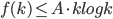 for k < n


 [what is left over]


 then
then 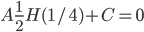 , so
, so
 Anlog(n) as claimed.
recursions: f(i)
on smaller part, larger part: f(n-i)
time to divide into smaller, larger: O(n)
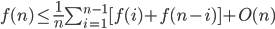
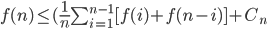
Claim: This implies: f(n) = O(n log n)
Have:
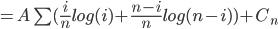
Want: f(n)
Inductive assumption:
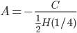
Define function H(x) = xlog(x) + (i-x)log(1-x) entropy function
for
H(1/4) < 0
Choose
Qsort supposed to be fastest, other faster ones are not too important.
Qsort libraries usually use middle element (how they even find middle element?) as pivot, not randomized, which is essential to qsort.
02/17/2016
Fast sorting Methods:
Mergesort: divide and conquer algorithm
quicksort: randomized algorithm
Heapsort: Use of data structure
Data Structure:
We give interface, it has to implement the given operations correctly, and as fast as possible.
Heap data structure: maintains a set of key values (or (key,object) pair).
Heapsort properties: insert, findmin, deletemin
Many ways to implement it. All with O(log n) for all operations.
Array-based heap
we store the elements currently in the heap in an array H[]
with properties:
1) we always us a prefix of H[] so if currently there are i elements in the heap, they are in posistions H[0]...H[i-1]
2) Heap order if there are i elements in the heap
then heap[j] <= heap[2*j+1] if 2j+1 <= i-1
heap[j] <=heap[2*j+2] 2j+2 <= i-1
Insert: If there are currently i elements, then by the no-gaps condition, new element needs to use first empty space H[i] but then in violates Heap order, so we exchange downard until heap order is satisfied. O(log n)
Deletemin: We have to remove the element at the bottom we also have to make the heap one element shorter (no gaps).
We have to restore heap order.
Classical method: move last element in the gap at the bottom,
then move it up until heap order is satisfied.
To move item H[j] up, we have to compare H[2j+1] and H[2j+2]
with H[j], if the smaller of H[j+1], H[2j+2] is smaller than H[j], exchange with that.
02/22/2016
See notes
02/24/2016
See notes
02/29/2016
Topological Sorting
Given a directed graph (vertices, directed edges)
We want to find a sequence of the vertices such that all edges go from earlier to later vertices (edges go from left to right)
Or show that no such sequence exists.
If there is a directed cycle, then no such sequence exists. If no such sequence exists, then there is a directed cycle.
Algorithm: Find a vertex with no incoming edges. Put that first, remove it from the graph. Repeat.
If there is no such vertex, then there is a directed cycle.
Suppose we have a directed graph in which each vertex has at least one incoming edge. Then this graph has a directed cycle.

 , that has occurred earlier
  .
.
Proof: Choose any starting vertex, and take its predecessor. Repeat: We get a sequence of vertices and edges.
This is an infinite sequence, but only finite number of vertices. There will be first vertex
we found directed cycle.
Algorithm (more detail)
Make a pass over all directed edges, keep track of indegree of each vertex (any of indegrees, initially 0, for edge i->j increment degree[j])
Took O(E)
make pass over all vertices, put vertices of indegree 0 on a stack. Took O(V).
Take a vertex from the stack (if not possible, with finite or no squence) put it next in output sequence. Take all edges from that vertex, O(E). Decrease indegree of their end vertices, if indegree is O. Put in stack.
Topological sorting can be done in O(E).
If the vertices are numbered: 0...v-1
(Else use such take or other dictionary structure to map vertex ID to number)
Median finding /Rank Order
We are given n items, and want to find the k-th largest of them. (k = n/2 median).
If we sort them, we can just look it up. But sorting takes O(n log n).
For k - 1, or k = n
We can answer in O(n).
What about other k?
Can be done in O(n) expected time for any k.
Algorithm Quickselect:
Want to find the k-th largest element of n given elements.
Select random comparison element (pivot) a[j], divide array into smaller and larger elements.
Let b be the number of i with a[i] < a[j].
If b < k we recursively search for the k-b smallest array items >= a[j]
Else, we search for the smallest array item < a[j].
Balanced Search Trees
(Height-balanced trees, leaf tree model)
*Leaf tree model: Data is stored only in the leaves, interior nodes just for left/right decision in nodes, no test for n -> key == query_key, only happens in the leaf.
*Node tree model: Each key comes with its data object, in each node test if n -> key == query_key.
Find question:
-Needs to encode when a node is a leaf
-Needs to store the associated data in the leaf.
Any convention of your choice.
Insert new key in the tree go down to the leaf where key should go.
There is already different key there. So,
- create two nodes (leaves) with old key new key. Make previous leaf if old_key < new_key.
- If old_key < new_key, then old_key leave goes left, new_key leaf goes right.
Key in new interior node is max(old_key, new_key).
03/02/2016
Balancing trees: rotations
Universal operations - a tree can be transformed in a ny other search tree with the same leaves and interior keys by rotation.
Want to show: a height balanced tree with n leaves has height O(log n)


 for some number > 1.
leaves(h) = minimum number of leaves of a height-balanced tree of height h
Want to show leaves(h) > b^n, for some b > 1
Minimal trees = Fibonacci Trees:
h = 0, 1 leaf
h = 1, 2 leaves
h = 2, 3 leaves
...
03/07/2016
Height Balanced Tree
Binary search tree: In each interior node the height of left subtree and the height of right subtree differ at most by one.
HBT: insert/delete possibly affect only height of nodes with changed leaf, not for other nodes.
Rotations of tree (for insertion/deletion)
03/09/2016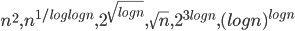

O-notation sorting functions according to growth rate
So: given some functions:
Sort them in increasing growth rate.
Given functions f(n), g(n)
then if lim f(n)/g(n) = +
then f(n) grows faster than g(n)
Things to remember (log n) grows slower than n
 for any constant K grows slower than n
if you have function with n in base and in exponent always try use everything to exponent.

Test Review:

Example: Given a function for which f(n+1) - f(n) = \Omega(n)
Ans:
Exponent 1: f(n) = n
n+1-n = 1 is not Ω(n)
Exponent 2: f(n) = (n)^2
(n+1)^2 - n^2 = 2n+1 = Ω(n)
Found: f(n) = n^2
Example: f(n) - f(n/2) = \Theta(1)
Ans: f(n) = log n
Bubblesort, insertion sort, selection sort (all O(n^2))
Mergesort, quicksort: O(n logn)
Heapsort: O(nlogn), insert/delete/find: O(logn)
Decision tree: Lower bound for comparison-based sorting
Linear time sorting with additional assumptions: counting sort, radix sort
Linear time median selection: topological sorting
Search Trees (leaf tree model)
Height-balanced search trees
03/28/2016
Graph Algorithms
1) Graph Exploration, Connectivity: Can we get there from here?
State Space Exploration
Graph: Given a start vertex. Methods to generate for each vertex its neighbor want to visit/generate all vertices that can be reaached from the start vertex.
(Directed graph: If u is generated as neighbor of v, it is not required (so far) that v is generated as neighbor of u)
BFS, uses queue
DFS uses a stack
both need a structure to maintain which vertices have been visited (search tree, hash table, bit field)
Algorithm: S start vertex given
put S on stack/in queue
while stack/queue not empty
{take vertex x from stack/queue
if (x not visited)
{mark x as visited,
generate all neighbor y_1...y_k of x
for each y_i, if (y_i is not visited) insert y_i on stack/in queue
}
}
Each vertex can be added to the queue once from each neighbor so upper bound for number of add-to-queue operations is \sum_v deg(v) = 2e
So there are \leq 2e add-to-queue operations so also \leq 2e remove from queue operations
So \leq 2e steps in total, where step includes
- operate a neighbor O(1)
- insert/delete from queue O(1)
- mark visited/check if visited O(1) or O(log n)
Total time of BFS/DFS:
O(e) if vertices are numbered
O(elog v) if vertices have arbitrary integer.
Why BFS works:
BFS generates/visits vertices in sequence of increasing distance from start vertex became queue has always this structure.
So we can get shortest paths from BFS
To use BFS to find shortest paths, we need to keep track in our queue for each vertex from where it was visited.
Get a tree of shortest paths pointing back to start vertex to find path from the start vertex, we have to invert the sequence. By putting it on a stack.
DFS without state copies:
On our stack we put the move, not the state
Needs undirected graph: every move allows an undo.
algorithm given
03/30/2016
Shortest paths in Graphs with Edge lengths
Do shortest paths exist? No if there are negative cycles, there are no shortest paths length can get as negative as we want.
If there are no negative cycles, then there are always shortest paths because assume we have a sequence of shorter and shorter paths )infinite sequence a) so paths got longer and longer. But we have only fixed number of vertices so they have to repeat some cycle again and again.
If there are no negative edges, then the algorithm of choice is Dijkstra's algorithm.
Give a graph with positive edgelengths and a start vertex s. We simultaneously compute shortest paths to all vertices of the graph.
Maintain for each vertex the length of the best path through finished vertices that we currently know.
Initially: s finished, dist(s) = 0
all neighbors v1...vk of s are boundary
dist(vi) = edgelength(s,vi)
Repeat until there are no boundary vertices left
{ take boundary vertex x with dist(x) minimal
change x to finished.
For each neighbor y of x
{if y is not finished) set y to boundary
dist(y) = min(dist(y), dist(x) + edgelength(x,y)
Dijkstra with loop:
v times: select from heap the smallest element => total O(vlogv)
\leq 2e times (for each neighbor) either - insert in heap O(logv) or - decrease distance in loop O(logv) => total O(elogv)
Total Time O(elogv)
04/04/2016
Minimum Spanning Trees
Undirected graph with edgelengths, edgelengths >= 0
We want the shortest subgraph that connects all vertices. Tree that connects all vertices.
Prim's Algorithm
Choose a start vertex (any)
Look at all out going edge of the current tree add the cheapest out going edge.
repeat until all is connected.
Need heap, need structure to keep track of visited vertice.
Choose start vertex, mark start vertex visited.
All others not visited.
Insert all outgoing edges of start vertex into heap repeat while heap not empty
{
take minimum weight edge ab from the heap
if a visited && b not visited
mark b visited, select edge ab for the tree, add all outgoing edges of b to the heap
else if b visited && a not visited
mark a visited.....
Analysis: Loop which enters and deletes each edge into/from the heap
each edge is at most twice enetered in the heap
(one from each end point)
entering/deleting from heap takes O(log V) time
Mark vertices as visited, look up visited status if done by search tree, takes O(log V)
do this for each edge so total O(ElogV)
Need to show correctness:
The tree that Prim's Algorithm produces is really the minimum spanning tree.
Assume the opposite: There is a spanning tree
whose total length is smaller than the tree Prim's algorithm
T_prim: tree produced by Prim's algorithm
T_opt: the minimum spanning tree
Assumption: length(T_opt) < length(T_prim)
Let ab be in edge in T_opt not in T_prim
Find such edges, so all edges chosen by Prim's algorithm before ab are also in T_opt.
1) Look up Minimum Spanning Tree, Prim's Algorithm in Wikipedia.
2) can fine tuen the algorithm, especially: should stop earlier. Should stop when all vertices are connected.
3) Krushkal's algorithm
04/06/2016
MST: Prim, Kruskal's Algorithm
Kruskal
Set union structure: root-directed trees
with union by rank
Each vertex gets one outgoing edge/pointer to another vertex
if that pointer is NULL, the vertex is a root.
Initially every vertex is root
Later: some vertices point to other vertices, and we can follow pointers until we find root.
Since component test for vertices u, v follow for both vertices the pointers until you find the root
if root(u) = root(v): same component
else: different component.
To join components containing vertices u, v
find root(u), root(v)
test that they are distinct point one to the other.
Each vertex gets an integer,
the rank: initially each rank = 0
We always point smaller root to larger root on joining
if they are the same, we increment the roots.
Along any path the ranks are increasing length of path <= maximum rank.
Component with root at rank k has at least 2^k vertices.
Complexity of same_component & join_component test is O(log v)
Kruskals Alg.:
First: sort the edges, takes O(E log E) = O(E log v)
then for each edge, do same-component test, possibly join components. O(E log v)
End of distance problem in Graphs
Next:
Maximum Flows on Graphs
bottleneck connections.
Graph directed capacities for each edge
Assign each edge a flow value.
1) Flow value is <= edge capacity
2) Flow value >= 0
3) for all vertices but s, t (source and target)
we have inflow = outflow
Flow preservation: sumflow(uv) = sum !flow(vu)
An assignment of flow values to directed edges that satisfies these conditions is a valid flow Maximum Flow problem
Maximize the flow from s to t
= maximum outflow of s in any valid flow.
Application in UPS?
04/11/2016
Maximum Flow Problems
Given a directed graph
each edge has a capacity
there are two special vertices s (source), t (sink)
aim maximize outflow of of s = inflow of t
A valid flow

assigns each directed edge a flow value
which is between O and capacity of the edge such that for each vertex (excluding s, t)
the inflow of the vertex = the outflow of the vertex
Idea of algorithm
Residual capacity graph
given a flow, the residual capacity graph represents the possible changes of the flow
Residual capacities in the original graph is replaced by two edges:
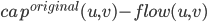
A new directed graph on the same vertex set (again a flow problem)
each edge
(u,v): forward edge, capacity
(v,u): backward edge, residual capacity: flow(u,v)
---------
if the original graph already had two edges (u,v) (v,u)
then we generate forward and backward edges for both, merge these in the same direction.
Cut: divide vertex set into two classes, one containing s, the other containing t.
Capacity of the cut:
The sum of edge capacities of edges going across the cut from s-side to the t-side
Since any flow from s to t has to flow across the cut for any flow, any cut capacity of cut separating s, t.
flow from s to t
Algorithm:
given capacities s, t
set initial flow to 0 on all edges
repeat {
construct the residual capacities graph
find a path from s to t with capacities > 0
increase the flow along that path by that minimum capacity
}
until no path is found. Then flow is maximal.
In the find residual capacities graph
there is no path from s to t,
so let X be the vertices that can be reached with capacities > 0 from S, and
Y be the remaining vertices
then X, Y is a cut separating s, t such that capacity of this cut = flow.
All edges going from X to Y has 0 reached capacity fully used
All edges from Y to X have 0 capacity on backward edge so not used at all.
Max flow min cut theorem
One iteration takes O(E)
each iteration increases flow value by at least 1
so number of iteration \leq maximum flow
so time O(E * maxflow)
if all edge capacities are \leq C
then outflow of s \leq CV, so time O(E*V)
This algorithm no good for NP problem.
Look up P-flow (push flow)
04/13/2016
May 18 Final
May 11 Final Review
Dynamic Programming
Example: Evaluate n-th Fibonacci number:
f(n) = f(n-1) + f(n-2), f(1)=f(2) = 1
Bad Idea
int f(int n)
{ if (n \leq 2) return(1);
else return (f(n-1)+f(n-2));
}
Total number of leaves in the call tree is f(n)~(16)^n
Second idea: Bottom up
Buttomupevaluation of f(n) takes O(n)
Top-down evaluation of f(n) takes ~(16)^n
Dynamic programming:
We are given a problem that can be decomposed into smaller problems of the same type.
Instead of recursively decomposing, we tabulate all small problems that can occur in this decomposition process,
then solve them from smallest to longest, reducing each problem to subproblems for which we already have the answer.
Complexity is determined by the number of subproblems we generate subproblems.
Subproblems are typically stored in a table, so this Dynamic Programming Table is feature of all DP algorithms.
Knapsack Problem
Given items 1 n item i has value a(1), weight b(1)
we can carry at most weight L, so which items should we select to maximize the value.
Subproblem[i,w]: maximum value we can achieve if the weight limit is w (1 \leq w \leq L) and we can use only items 1, ..., i
first column: subproblem [1,w] =
a). O(1) if w \geq b(1)
b). O else
fill in column i+1, column 1...i already finished
subproblem [i+1, w] =
a). max(a(i+1)+subproblem(i,w-b(i)), subproblem(i,w)), if b(i+1) \leq w
b). subproblem(i,w), else
Complexity of finding subproblem(n,L) (our original problem) in O(1) per table entry, So O(n+L)
Knapsack Complexity: size of the table
Edit distance of Strings
Define edit operations:
insert a character
delete a character
exchange one character for another
distance of two strings is the minimum cost sequence of edit operations that changes on string to the other.
Edit distance of s_1...s_n to t_1...t_m insert cost(t_k)
 delete cost(s_k)
subproblem[i,j] = edit distance of s_1...s_i to t_1...t_j
subproblem[0,j] = edit distance from empty string to t_1...t_j =
subproblem[i,0] = edit distance from s_1...s_i to emptystring =
For i,j \geq 1
subproblem[i,j] = min {
subproblem[i-1,j] + deletecost(s_i),
subproblem[i,j-1] + insert cost(t_j),
subproblem[i-1,j-1] + exchangecost(s_i,t_j)
}
Complexity of....subproblem(n,m) = the original problem is O((mn)
This is not just useful with dictionary, but also in Bioinformatics.
04/18/2016
Floyd-Warshall all pairs shortest path
Look up details.
F-W algorithm needs O(V^3) time
Space can be reduced to O(V^2)
because S[i,j,k-1] is not needed after s[ijk]
F-W code:
{ create table S[n][n][n+1]
for (i = 1...n) for (j = 1...n) if (edge vec(i,j) exist)
{
S[i,j,0] = edgelength(vec(i,j));
else S[i,j,0] = +infinity;
}
for (k = 1...n) for (i = 1...n)
s[i,j,k] = min(S[i,j,k-1], S[i,k,k-1]+S[k,j,k-1])
}
Single-source shortest path with negative edgelengths alllowed
Bellman-Ford algorithm
(similar to Dijkstra, but easier)
Coin change problem
04/20/2016
Complexity Classes
Up to now: studied complexity of algorithms
next: complexity of problems
Sample problems:
1. sorting n numbers
2. find minimum spanning tree
3. Find shortest path
4. find the shortest closed walk that visits each vertex(traveling salesman problem)
5. Assign three colors to vertices of a graph so that neighboring vertices have different colors
Decision Problems: Problems with yes/no answer
Sample problems:
1. Is the minimum spanning tree length \leq k
2. can the graph be 3-colored
3. does the graph have a hamiltonian circuit (cycle visits each vertex exactly once)
4. can a given boolean formula be satisfied?
Class P: decision problems for which an algorithm exists that solves each problem of size n in O(n^C) time, C is some constant.
Polynomial time Algorithms
Leads to P = NP problem
Class NP: Those decision problems for which algorithm exists that takes problem instance (size n)
and additional O(n^C) but of evidence as input and
if the answer to problem is yes
then for some evidence the algorithm will answer "yes"
if the answer to problem is no
then for any evidence the algorithm will answer "no"
and algorithm run in O(n^C) time
Class NP: Problems for which a "yes" answer can be checked in polynomial time, given some certificate of polynomial length (Some ways to satisfy "yes" answer)
Example: boolean function satisfiable: is in NP.
Since given the satisfying assignment we can check it
and any non-satisfying assignment will be rejected.
Sample problems of NP:
Satisfiability Problem (SAT)
1. Graph 3-colorability
2. Hamiltonian Circuit
3. Maximum Independent set
P \subseteq NP
famous problem is P = NP
PhD level, unsolved.
Unknown problem: P = NP = P-Space = Exptime, Polynomial collapse
There appears to be a movie about this.
Reducibility of Problems
I have two problems, Pr_1, Pr_2
and any instance of Pr_1 can be reduced by some polynomial-time preprocessing to an instance of Pr_2 with the same answer.
If I can solve Pr_2 in polynomial time, then I can solve Pr_1 in polynomial time.
If Pr_1 cannot be solved in polynomial time,
then Pr_2 cannot be solved in polynomial time.
So, Pr_1 reduced in polynomial time to Pr_2
then Pr_2 is at least as hard as Pr_1
A Problem is NP-Complete
If every problem in NP can be reduced to it.
Theorem: SAT is NP-complete
Proven
Outline of prof's proof:
We want to show: any problem in NP can be reduced to SAT
How is a problem in NP given?
Problem is given as a piece of code that takes problem instance and additional certificate, answer yes/no
Need to transform:
-that piece of code
-Problem instance of size n into a boolean satisfiability problem with same answer.
That piece of code takes O(n^C) to execute on problem size n,
so it needs only O(n^C) storage/memory.
Model the possible execution of that piece of code on a computer
O(n^C) boolean variable corresponding to the memory cells.
Each variable exists in O(n^C) copies, for the O(n^C) time steps
Table: time step (y-axis), O(n^C) X memory addresses (x-axis, O(n^C)
O(n^{2C}) boolean variables in total.
Count each variable from one timestep to the next.
Can model the possible transition from one step to next also as boolean formula.
Get: Boolean formula of size O(n^{2C}) that describes all possible executions of program on input put in the memory cells at time 0.
Assign the problem instance to the problem input bits, leave certificate bits open.
Then ask SAT solver "are there any certificate bits such that the program run will end with yes?"
If answer is yes, then answer to original problem is yes, else no.
So, SAT instance has same answer as original problem.
For samples of NP complete problems, Prof recommended this book.
Finite Automata = Finite Automaton = Finite State Machine (FSM)
Turing Machine
05/02/2016
Arithmetic on Long Integers
- addition, no problem, add 2 n bit numbers, O(n)
- subtraction, same
- multiplication, normal style O(n^2) => Karatsuba Algorithm
- division, can be done O(time of multiplication)
- exponentiation
- modulo a number
Karatsuba-Ofen algorithm for multiplication of n-bit #
Idea: multiply recursively reduce n-bit multiplication to n/2 bit multiplication
A x B, A, B n bit numbers
A = A_upper * 2^(n/2) + A_lower
B = B_upper * 2^(n/2) + B_lower
A_upper B_upper upper n/2 bits
A_lower B_lower lower n/2 bits
AxB = A_upper * B_upper * 2^n + A_upper * B_lower * 2^(n/2) + A_lower * B_upper * 2^(n/2) + A_lower * B*lower * 2^0
----
So one n-bit multiplication reduced to four n/2 bit multiplication, some shifts, some additions
t(n) \leq 4t(n/2) + O(n)
Recursion gives t(n) = O(n^2).
Need to rewruite the 4 terms so that only three multiples necessary.
Karatsube-Ofen (ofman?) Algorithm:
Sum1 = A_upper + A_lower
Sum2 = B_upper + B_lower
Prod1 = Sum1 * Sum2 = A_upper * B_upper + A_upper * B_lower + A_lower * B_upper + A_lower * B_lower
Prod2 = A_upper * B_upper
Prod3 = A_upper * B_lower
Thus,
A*B = Prod2 * 2^n + (Prod1 - Prod2 - Prod3) * 2^(n/2) + Prod3 * 2^0
Reduced n-bit multiplication to 3 n/2 bit multiplication and addition, subtraction, shifts
t(n) \leq 3t(n/2) * n/2 + O(n), => t(n) \leq O(n^{log 3})
Fourier's Transform mentioned.
Polynomial interpolation mentioned!
Basic operation in Cryptography (RSA)
a^b mod c
a,b,c are long integers
First attempt: compute a^b as a*a*...*a, b times
takes O(b) where b is long int 2^1024
Not possible!
Better way: reduce to O(log b) multiplications (after each mult, reduce mod c)
Example: (123)^456 = ((123)^2)^228 = ... = ((((123)^2)^2)^2)57 = let it = A(A)^56 = A*(A^2)^28...
= A(((A^2)^2)^2)^7
= A*B*B^6 = A*B(B^2)^3 = AB^B*B^2*((B^2)^2)
So, need only < 2(log b) multiplication to compute a^b
Next, Newton's Method:
given f,
want to find x such that f(x) = 0
05/04/2016
Algorithms on Strings
linear time string matching
Given two strings s and t. We want to decide whether s is a substring of t.
m = length(s), n = length(t)
Does there exist an i such that for j = 0...(m-1)
s[j] = t[i+j]
Start recording...
self overlaps of s
...prefix_k(x) = suffix_k(x)
...outline how to construct table of maximal self-overlaps of prefixes of s
05/09/2016
Traveling Salesman Problem TSP
Given n cities that have to be visited.
With their distances, find the closed tour which visits all cities exactly once, and has minimal cost.
Given a graph with edge lengths.
Want the cycle through all vertices of the graph of minimum cost.
Assume that the edge lengths satisfy the triangle inequality d(a,c) \leq d(a,b) + d(b,c).
Trivial algorithm for exact solution:
closed tour has to include vertex 1.
cut it open at vertex 1, then the other n-1 vertices are visited in some sequence. Try all (n-1)! seq. complexity O((n-1)!), unreasonable even for n = 10.
Better exact algorithm (Held-Karp-Algorithm
Dynamic programming idea:
Tabulate the shortest path that starts at vertex 1,
ends at vertex i, uses vertex set S with 1, i \subset S \subseteq \{1,...,n\}
Do this for all S, and all i \in S
TSP is NP-Complete
Contains a special case Hamiltonian circuit problem (given a graph, i, these closed tour which visits each vertex exactly once?)
Hamiltonian circuit is also NP complete.
apparently difficult problems, Yet large instances have been solved exactly.
- There are easy instances
- in any problem instance, main difficulty is to show that the proposed solution is optimal.
There are some techniques to generate lower bounds for TSP instance, if the lower bound meets the length of the given tour, then the given tour is optimal.
One lower bound technique 'rivers and moats'
Approximation algorithm for TSP
Choose a minimum spanning tree (MST) go around the tree, skipping vertices you have already visited before.